3.8 Comparison of Importance Sampling Methods - Figures

library(here)
source(here("setup.R"))

df_are_mu <- read_csv(here("data/figures/are_mu.csv"))
df_are_sigma2 <- read_csv(here("data/figures/are_sigma2.csv"))

df_rho_ce_sigma2 <- read_csv(here("data/figures/rho_cem_sigma2.csv"))
df_rho_eis_sigma2 <- read_csv(here("data/figures/rho_eis_sigma2.csv"))
df_rho_mu <- read_csv(here("data/figures/rho_mu.csv"))

rename_scenario <- function(df) {
    df %>% rename(
        "$\\mathcal N (0, 1)$" = 2,
        "loc. mixture, $\\omega^2 = 0.1$" = 3,
        "loc. mixture, $\\omega^2= 0.5$" = 4,
        "loc. mixture, $\\omega^2 = 1$" = 5,
        "scale mixture, $\\varepsilon^2 = 100$" = 6,
        "scale mixture, $\\varepsilon^2 = 10$" = 7,
        "scale mixture, $\\varepsilon^2 = 2$" = 8
    )
}

add_type <- function(df) {
    df %>%
        mutate(type_short = str_sub(name, 1, 3)) %>%
        mutate(type = case_when(
            type_short == "$\\m" ~ "normal",
            type_short == "loc" ~ "location mixture",
            type_short == "sca" ~ "scale mixture"
        )) %>%
        mutate(type = factor(type, levels = c("normal", "location mixture", "scale mixture")))
}

here() starts at /Users/stefan/workspace/work/phd/thesis

tikz/are.tex

df_are_mu_fig <- df_are_mu %>%
    rename_scenario() %>%
    pivot_longer(-sigma2) %>%
    add_type()

df_are_sigma2_fig <- df_are_sigma2 %>%
    rename_scenario() %>%
    pivot_longer(-mu) %>%
    add_type()


plt_mu <- df_are_mu_fig %>%
    mutate(name = str_extract(name, "\\$.*\\$")) %>%
    ggplot(aes(sigma2, value, linetype = name, color = type)) +
    geom_line() +
    coord_cartesian(ylim = c(1e-2, 1e2)) +
    scale_y_log10(breaks = 10^(-2:2), labels = paste0("$10^{", -2:2, "}$")) +
    scale_linetype_discrete(name = "") +
    scale_color_discrete(name = "") +
    labs(x = "$\\sigma^2$", y = "$\\frac{V_{EIS}}{V_{CE}}$")

plt_sigma2 <- df_are_sigma2_fig %>%
    mutate(name = str_extract(name, "\\$.*\\$")) %>%
    ggplot(aes(mu, value, linetype = name, color = type)) +
    geom_line() +
    coord_cartesian(ylim = c(1e-2, 1e2)) +
    scale_y_log10(breaks = 10^(-2:2), labels = paste0("$10^{", -2:2, "}$")) +
    scale_linetype_discrete(name = "") +
    scale_color_discrete(name = "") +
    labs(x = "$\\mu$", y = "$\\frac{V_{EIS}}{V_{CE}}$")

(plt_mu | plt_sigma2) + plot_layout(guides = "collect") &
    theme(legend.position = "bottom")

ggsave_tikz(here("tikz/are.tex"))

Warning message in scale_y_log10(breaks = 10^(-2:2), labels = paste0("$10^{", -2:2, :

“log-10 transformation introduced infinite values.”

Warning message in scale_y_log10(breaks = 10^(-2:2), labels = paste0("$10^{", -2:2, :

“log-10 transformation introduced infinite values.”

Warning message in scale_y_log10(breaks = 10^(-2:2), labels = paste0("$10^{", -2:2, :

“log-10 transformation introduced infinite values.”

Warning message in scale_y_log10(breaks = 10^(-2:2), labels = paste0("$10^{", -2:2, :

“log-10 transformation introduced infinite values.”

pdf: 2

tikz/rho.tex

df_rho_ce_fig <- df_rho_ce_sigma2 %>%
    rename_scenario() %>%
    pivot_longer(-mu) %>%
    add_type() %>%
    mutate(name = str_extract(name, "\\$.*\\$")) %>%
    rename("rho" = value) %>%
    mutate("EF" = 1 / rho * 100)
df_rho_eis_fig <- df_rho_eis_sigma2 %>%
    rename_scenario() %>%
    pivot_longer(-mu) %>%
    add_type() %>%
    mutate(name = str_extract(name, "\\$.*\\$")) %>%
    rename("rho" = value) %>%
    mutate("EF" = 1 / rho * 100)

scales_fig <- list(
    scale_linetype_discrete(name = ""),
    scale_color_discrete(name = "")
)


p1 <- df_rho_ce_fig %>%
    ggplot(aes(mu, EF, color = type, linetype = name)) +
    geom_line() +
    labs(x = "$\\mu$", y = "EF [\\%]") +
    scales_fig +
    coord_cartesian(ylim = c(0, 100)) +
    ggtitle("CE-method")
p2 <- df_rho_eis_fig %>%
    ggplot(aes(mu, EF, color = type, linetype = name)) +
    geom_line() +
    labs(x = "$\\mu$", y = "EF [\\%]") +
    scales_fig +
    coord_cartesian(ylim = c(0, 100)) +
    ggtitle("EIS")

p3 <- select(rename(df_rho_ce_fig, "CE" = "EF"), -rho) %>%
    inner_join(select(rename(df_rho_eis_fig, "EIS" = "EF"), -rho)) %>%
    mutate(`relative EF` = CE / EIS) %>%
    ggplot(aes(mu, `relative EF`, color = type, linetype = name)) +
    geom_line() +
    coord_cartesian(ylim = c(NA, 1.5)) +
    scales_fig +
    xlab("$\\mu$") +
    ylab("relative EF (CE/EIS)")


(p1 | p2 | p3) + plot_layout(guides = "collect") & theme(legend.position = "bottom")

ggsave_tikz(here("tikz/rho.tex"))

Joining with `by = join_by(mu, name, type_short, type)`

pdf: 2

tikz/rho_mu.tex

df_rho_mu %>%
    rename_scenario() %>%
    pivot_longer(-sigma2) %>%
    add_type() %>%
    mutate(name = str_extract(name, "\\$.*\\$")) %>%
    rename("rho" = value) %>%
    mutate("EF" = 1 / rho * 100) %>%
    ggplot(aes(sigma2, EF, color = type, linetype = name)) +
    geom_line() +
    labs(x = "$\\sigma^2$", y = "EF [\\%]") +
    scale_color_discrete(name = "") +
    scale_linetype_discrete(name = "") +
    theme(legend.position = "bottom")

ggsave_tikz(here("tikz/rho_mu.tex"))

Warning message:

“Removed 5 rows containing missing values or values outside the scale range

(`geom_line()`).”

Warning message:

“Removed 5 rows containing missing values or values outside the scale range

(`geom_line()`).”

pdf: 2

tikz/cem_eis_sigma2.tex

cem_sigma2 <- read_csv(here("data/figures/cem_sigma2.csv")) %>%
    rename_scenario() %>%
    pivot_longer(-mu) %>%
    add_type() %>%
    mutate(name = str_extract(name, "\\$.*\\$")) %>%
    rename(sigma2 = value) %>%
    mutate(method = "CE")

eis_sigma2 <- read_csv(here("data/figures/eis_sigma2.csv")) %>%
    rename_scenario() %>%
    pivot_longer(-mu) %>%
    add_type() %>%
    mutate(name = str_extract(name, "\\$.*\\$")) %>%
    rename(sigma2 = value) %>%
    mutate(method = "EIS")

cem_sigma2 %>%
    rbind(eis_sigma2) %>%
    ggplot(aes(mu, sigma2, color = type, linetype = name)) +
    geom_line() +
    facet_wrap(~method, scales = "free_y") +
    coord_cartesian(ylim = c(0, 3)) +
    labs(x = "$\\mu$", y = "$\\sigma^2$") +
    scale_color_discrete(name = "") +
    scale_linetype_discrete(name = "") +
    theme(legend.position = "bottom")

ggsave_tikz(here("tikz/cem_eis_sigma2.tex"))

pdf: 2

tikz/gssm_eps.tex

df_eps <- read_csv(here("data/figures/gsmm_eps.csv"))

p1 <- df_eps %>%
    select(epsilon, sigma2_cem, sigma2_eis) %>%
    pivot_longer(-epsilon, names_pattern = "sigma2_(.*)", values_to = "sigma2") %>%
    mutate(name = ifelse(name == "cem", "CE", "EIS")) %>%
    ggplot(aes(epsilon**2, sigma2 - (1 / 2 + 1 / 2 / epsilon**2), color = name)) +
    geom_line() +
    scale_x_log10() +
    # scale_y_log10() +
    scale_color_discrete(name = "") +
    labs(x = "$\\varepsilon^2$", y = "$\\hat \\sigma^2 - (\\frac 1 2 + \\frac 1 {2\\varepsilon^2})$") +
    ylim(-10, 5)

p2 <- df_eps %>%
    select(epsilon, starts_with("rho")) %>%
    pivot_longer(-epsilon, names_pattern = "rho_(.*)", values_to = "rho") %>%
    mutate(name = ifelse(name == "cem", "CE", "EIS")) %>%
    ggplot(aes(epsilon**2, 1 / rho * 100, color = name)) +
    geom_line() +
    scale_x_log10() +
    labs(x = "$\\varepsilon^2$", y = "EF [\\%]") +
    scale_color_discrete(name = "") +
    ylim(0, 100)

p3 <- df_eps %>%
    select(epsilon, are) %>%
    ggplot(aes(epsilon**2, are)) +
    geom_line() +
    scale_x_log10() +
    labs(x = "$\\varepsilon^2$", y = "$V_{EIS} / V_{CE}$") +
    theme(legend.position = "bottom")

(p1 / p2 / p3) + plot_layout(guides = "collect") & theme(legend.position = "bottom")
ggsave_tikz(here("tikz/gsmm_eps.tex"))

Warning message:

“Removed 19 rows containing missing values or values outside the scale range

(`geom_line()`).”

Warning message:

“Removed 24 rows containing missing values or values outside the scale range

(`geom_line()`).”

Warning message:

“Removed 19 rows containing missing values or values outside the scale range

(`geom_line()`).”

Warning message:

“Removed 24 rows containing missing values or values outside the scale range

(`geom_line()`).”

pdf: 2

tikz/targets.tex

types <- c("normal", "location mixture", "scale mixture")
to_type <- function(label) factor(label, levels = types)

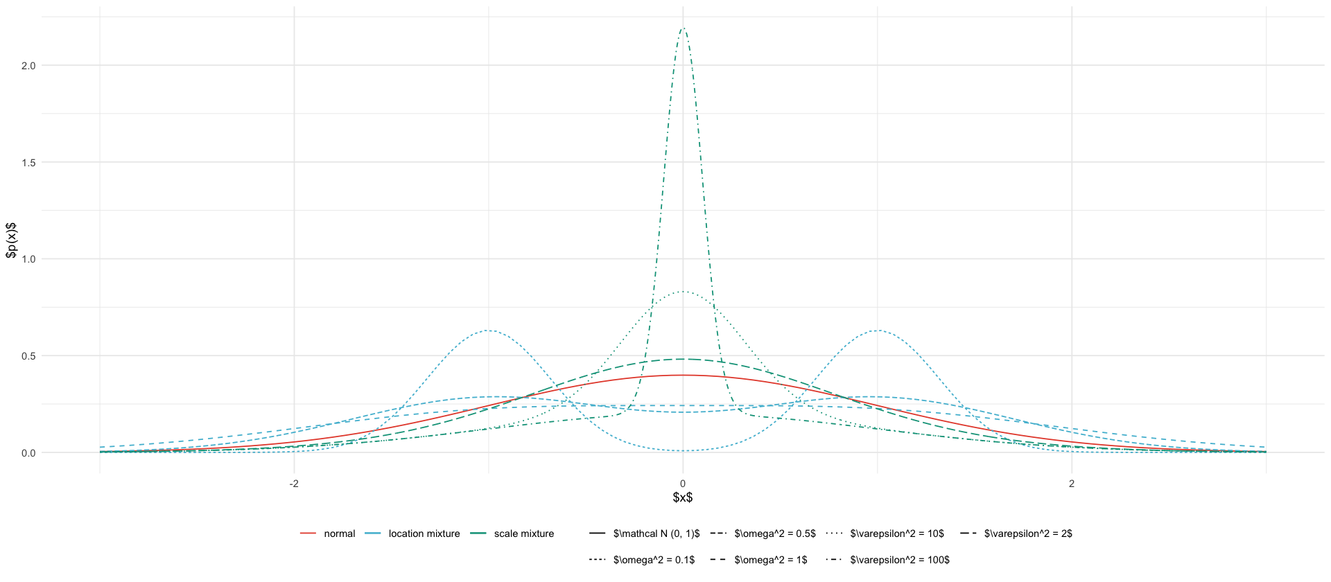
# Define the location mixture function
location_mixture <- function(x, omega2) {
    0.5 * dnorm(x, mean = -1, sd = sqrt(omega2)) +
        0.5 * dnorm(x, mean = 1, sd = sqrt(omega2))
}


omega2s <- c(0.1, 0.5, 1.0)
loc_geoms <- map(
    omega2s, 
    ~geom_function(fun = function(x) location_mixture(x, omega2 = .x), aes(color=to_type("location mixture"), linetype=paste0("$\\omega^2 = ", .x, "$")))
)

# Define the scale mixture function
scale_mixture <- function(x, eps2) {
    .5 * dnorm(x, mean=0, sd=1) + .5 * dnorm(x, mean=0, sd=sqrt(1/eps2))
}

eps2s <- c(2, 10, 100)
scale_geoms <- map(
    eps2s, 
    ~geom_function(fun = function(x) scale_mixture(x, eps2 = .x), aes(color=to_type("scale mixture"), linetype=paste0("$\\varepsilon^2 = ", .x, "$")), n= 1001)
)

ggplot() +
    geom_function(fun = dnorm, aes(color = to_type("normal"), linetype = "$\\mathcal N (0, 1)$")) +
    loc_geoms +
    scale_geoms +
    xlim(-3, 3) +
    labs(color = "Distribution", linetype = "Parameter") +
    scale_color_discrete(name = "") +
    scale_linetype_discrete(name = "") +
    theme_minimal() +
    theme(legend.position = "bottom") +
    labs(x = "$x$", y = "$p(x)$", color = "target", linetype = "parameter")

ggsave_tikz(here("tikz/targets.tex"))

pdf: 2