ssm_comparison_figures

library(here)

source(here("setup.R"))

here() starts at /Users/stefan/workspace/work/phd/thesis

df_ef <- read_csv(here("data/figures/ef_meis_cem_ssms.csv"))

# count missing values per column on df_ef
df_ef %>%
    select(n, LA=EF_LA,EIS=EF_MEIS, CEM=EF_CEM) %>%
    group_by(n) %>%
    summarise(across(everything(), ~ sum(is.na(.)))) %>%
    kable(format="latex", booktabs=TRUE, linesep="") %>%
    cat(., file=here("tables/ssm_comparison_missing_values.tex"))

unique_n <- df_ef$n %>% unique() %>% sort()
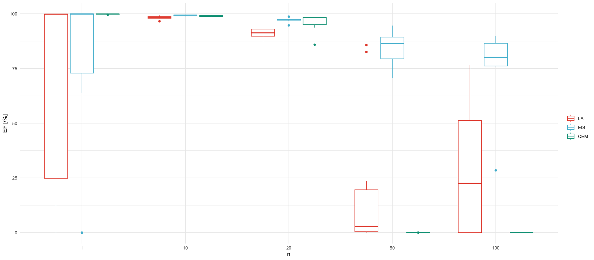
p_ef <- df_ef %>%
    select(n, LA=EF_LA, CEM=EF_CEM, EIS=EF_MEIS) %>%
    pivot_longer(-n, names_to = "Method", values_to = "EF") %>%
    mutate(Method = factor(Method, levels=c("LA", "EIS", "CEM"))) %>%
    ggplot(aes(x = factor(n), y = EF, color = Method, group=interaction(factor(n), Method))) +
    geom_boxplot() +
    labs(x = "n", y = "EF [\\%]", color="")

ggsave_tikz(
    here("tikz/ssm_comparison_efficiency_factor.tex"),
    plot = p_ef
)
p_ef

Warning message:

“Removed 26 rows containing non-finite outside the scale range

(`stat_boxplot()`).”

pdf: 2

Warning message:

“Removed 26 rows containing non-finite outside the scale range

(`stat_boxplot()`).”

df_are

A spec_tbl_df: 40 × 6
n	N_samples	N_iter	DET_CEM	DET_MEIS	ARE
<dbl>	<dbl>	<dbl>	<dbl>	<dbl>	<dbl>
1	10000	1000	1.250198e-21	7.362585e-21	1.698042e-01
1	10000	1000	2.131546e-19	7.124898e-18	2.991686e-02
1	10000	1000	1.520778e-20	6.692526e-20	2.272353e-01
1	10000	1000	6.007386e-17	6.660607e-11	9.019277e-07
1	10000	1000	6.624824e-22	3.177769e-22	2.084741e+00
1	10000	1000	1.151610e-21	3.231204e-21	3.564029e-01
1	10000	1000	3.083249e-23	1.207182e-22	2.554088e-01
1	10000	1000	3.179683e-21	4.044667e-21	7.861420e-01
1	10000	1000	2.180299e-18	8.979118e-15	2.428188e-04
1	10000	1000	1.877286e-20	2.278412e-18	8.239452e-03
2	10000	1000	1.927399e-28	1.079899e-28	1.784796e+00
2	10000	1000	1.144634e-32	2.888226e-32	3.963103e-01
2	10000	1000	6.159994e-29	7.289892e-29	8.450048e-01
2	10000	1000	1.429030e-31	2.081389e-32	6.865755e+00
2	10000	1000	5.423362e-30	7.953996e-30	6.818413e-01
2	10000	1000	5.877860e-32	6.436372e-32	9.132256e-01
2	10000	1000	5.379362e-33	1.062051e-32	5.065069e-01
2	10000	1000	4.887804e-31	5.855831e-30	8.346902e-02
2	10000	1000	2.035986e-32	9.830573e-32	2.071076e-01
2	10000	1000	7.752964e-33	9.875676e-34	7.850566e+00
5	10000	1000	1.306769e-54	3.883234e-60	3.365157e+05
5	10000	1000	7.110526e-50	1.654847e-59	4.296787e+09
5	10000	1000	3.682259e-69	7.342128e-71	5.015248e+01
5	10000	1000	1.271453e-57	3.366841e-62	3.776399e+04
5	10000	1000	1.589256e-62	2.441037e-65	6.510576e+02
5	10000	1000	7.400743e-67	5.401150e-68	1.370216e+01
5	10000	1000	1.671573e-55	2.222286e-61	7.521860e+05
5	10000	1000	6.099313e-58	1.303119e-63	4.680551e+05
5	10000	1000	9.018652e-68	1.924074e-70	4.687269e+02
5	10000	1000	2.414396e-61	8.786312e-65	2.747906e+03
10	10000	1000	1.052184e-139	-3.827550e-153	-2.748974e+13
10	10000	1000	-1.867709e-124	5.903577e-146	-3.163691e+21
10	10000	1000	-7.623069e-129	1.299750e-146	-5.865026e+17
10	10000	1000	3.335174e-127	-7.751308e-148	-4.302724e+20
10	10000	1000	-2.491652e-142	-3.458454e-152	7.204527e+09
10	10000	1000	-9.698239e-153	2.342988e-159	-4.139262e+06
10	10000	1000	-4.840100e-124	7.639541e-146	-6.335590e+21
10	10000	1000	-8.222822e-109	-4.968050e-143	1.655141e+34
10	10000	1000	-5.209369e-142	-7.930262e-154	6.568975e+11
10	10000	1000	-7.507561e-142	4.376430e-155	-1.715453e+13

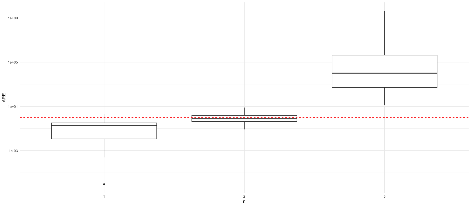
df_are <- read_csv(here("data/figures/are_meis_cem_ssms.csv"))
p_are <- df_are %>%
    filter(n <= 5) %>%
    ggplot(aes(x = factor(n), y = ARE)) +
    geom_boxplot() +
    labs(x = "n", y = "ARE", color="") +
    geom_hline(yintercept = 1, linetype="dashed", color = "red") +
    scale_y_log10() 

ggsave_tikz(
    here("tikz/ssm_comparison_asymptotic_variance.tex"),
    plot = p_are
)
p_are

pdf: 2