library(here)
source(here("setup.R"))Figures
Showcase
Parameters
theta_showcase <- read_csv(here("data/results/4_showcase_model/thetas.csv")) %>%
    rename("\\rho" = 2)

standard_errors <- read_csv(here("data/results/4_showcase_model/standard_errors.csv"))
standard_errors

variances <- theta_showcase %>%
    mutate(across(where(is.numeric), ~ exp(.x)))

sds <- variances %>%
    mutate(across(where(is.numeric), ~ sqrt(.x)))
sds

var_log_M <- variances %>%
    filter(method == "MLE") %>%
    pull(M)

var_M <- exp(var_log_M) - 1
sd_M <- sqrt(var_M)

c("var_M" = var_M, "sd_M" = sd_M)| parameter | standard_error |
|---|---|
| <chr> | <dbl> |
| log_rho | 0.0003029599 |
| W | 0.0004857571 |
| q | 0.0232959030 |
| M | 0.0028312903 |
| W_q | 0.0399133839 |
| method | \rho | W | q | M | W_q |
|---|---|---|---|---|---|
| <chr> | <dbl> | <dbl> | <dbl> | <dbl> | <dbl> |
| manual | 0.00100000 | 0.10000000 | 0.5000000 | 0.0100000 | 0.1000000 |
| initial | 0.01482601 | 0.02379713 | 0.1203075 | 0.1360824 | 0.8124226 |
| MLE | 0.01482571 | 0.02379714 | 0.1208721 | 0.1360977 | 0.8133194 |
- var_M
- 0.0186951937455615
- sd_M
- 0.136730368775783
tables/showcase-parameters.tex
# use scientific notation
sds_renamed <- sds %>%
    rename_with(function(col) str_glue("$\\hat\\sigma_{{ {col} }}$"), where(is.numeric))

sds_renamed %>%
    kable(format = "latex", format.args = list(scipen = 2, digits = 2), booktabs = T, escape = F) %>%
    cat(., file = here("tables/showcase-parameters.tex"))
Raw data
rep_tri <- read_csv(here("data/processed/RKI_4day_rt.csv"))Predictions
df_showcase <- read_predictions(
    here("data/results/4_showcase_model/predictions.npy"),
    seq(ymd("2020-04-05"), ymd("2020-09-01"), by = "1 day"),
    c("I", "I_corrected", "$\\rho$", "M", "W", "running_W", "$p^s_1$", "$p^s_2$", "$p^s_3$", "$p^s_4$", "$p_1$", "$p_2$", "$p_3$", "$p_4$", "$W_{q_1}", "W_{q_2}", "W_{q_3}")
)
figures/showcase_prediction_intervals_I_rho.tex
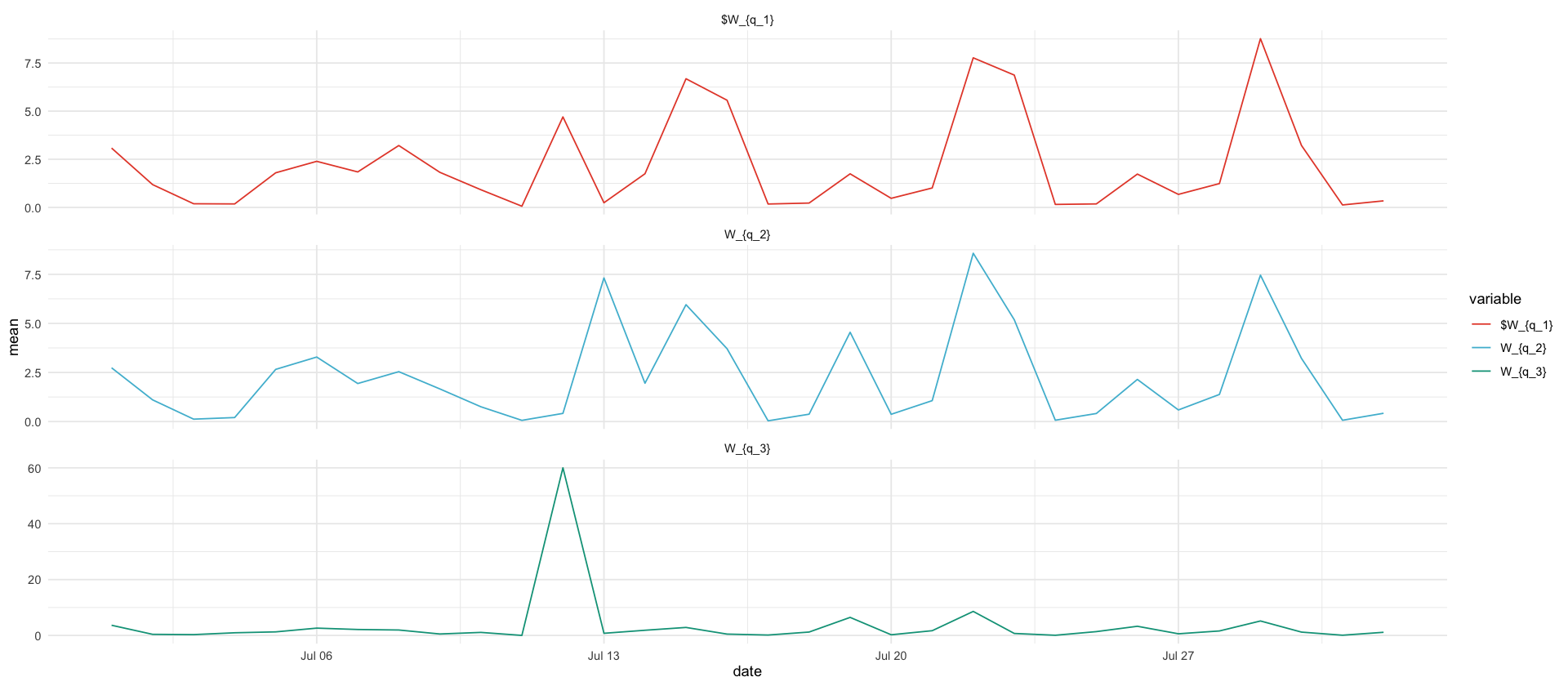
df_showcase %>%
    filter(variable %in% c("$W_{q_1}","W_{q_2}", "W_{q_3}")) %>%
    filter(date >= ymd('2020-07-01'), date <= ymd("2020-08-01")) %>%
    ggplot(aes(date, mean, color=variable)) +
    geom_line() +
    #scale_y_log10() +
    facet_wrap(~variable, ncol=1, scales="free_y")

rep_tri %>%
filter(county_date >= ymd('2020-07-01'), county_date <= ymd("2020-08-01"))| county_date | 1 | 2 | 3 | 4 |
|---|---|---|---|---|
| <date> | <dbl> | <dbl> | <dbl> | <dbl> |
| 2020-07-01 | 300 | 138 | 25 | 0 |
| 2020-07-02 | 298 | 143 | 7 | 7 |
| 2020-07-03 | 256 | 87 | 28 | 31 |
| 2020-07-04 | 141 | 88 | 51 | 14 |
| 2020-07-05 | 75 | 63 | 1 | 1 |
| 2020-07-06 | 170 | 125 | 11 | 0 |
| 2020-07-07 | 236 | 134 | 18 | 1 |
| 2020-07-08 | 299 | 131 | 12 | 2 |
| 2020-07-09 | 263 | 140 | 6 | 1 |
| 2020-07-10 | 221 | 112 | 21 | 0 |
| 2020-07-11 | 129 | 81 | 0 | 64 |
| 2020-07-12 | 55 | 0 | 75 | 1 |
| 2020-07-13 | 10 | 303 | 7 | 1 |
| 2020-07-14 | 224 | 199 | 28 | 3 |
| 2020-07-15 | 303 | 208 | 14 | 1 |
| 2020-07-16 | 351 | 171 | 3 | 3 |
| 2020-07-17 | 345 | 50 | 32 | 68 |
| 2020-07-18 | 139 | 159 | 80 | 17 |
| 2020-07-19 | 55 | 98 | 19 | 2 |
| 2020-07-20 | 257 | 124 | 10 | 24 |
| 2020-07-21 | 276 | 177 | 41 | 13 |
| 2020-07-22 | 381 | 259 | 38 | 1 |
| 2020-07-23 | 445 | 209 | 4 | 0 |
| 2020-07-24 | 488 | 138 | 19 | 92 |
| 2020-07-25 | 162 | 232 | 110 | 26 |
| 2020-07-26 | 106 | 81 | 19 | 1 |
| 2020-07-27 | 309 | 168 | 26 | 13 |
| 2020-07-28 | 400 | 279 | 50 | 9 |
| 2020-07-29 | 561 | 303 | 33 | 1 |
| 2020-07-30 | 488 | 318 | 19 | 7 |
| 2020-07-31 | 523 | 181 | 39 | 147 |
| 2020-08-01 | 233 | 197 | 90 | 26 |
fmt_numbers <- function(x) {
  s <- formatC(x, format = "f", big.mark = ",", digits = 0)
  gsub(",", "\\\\,", s)  # escape backslash for LaTeX
}

delta_t <- 4
df_corrected <- df_showcase %>%
    filter(date >= min(date) + delta_t, date <= max(date) - delta_t) %>%
    filter(variable %in% c("I_corrected", "I")) %>%
    group_by(variable) %>%
    summarize(total = sum(mean)) %>%
    rbind(
    rep_tri %>%
        filter(county_date <= max(df_showcase$date) - delta_t, county_date >= min(df_showcase$date) + delta_t) %>%
        summarize(total = sum(`1` + `2` + `3` + `4`)) %>%
        mutate(variable="truth")
    ) %>%
    mutate(
        header = case_when(
            variable == 'I' ~ "$\\sum_{t = 4}^{T-4} I_t$",
            variable == 'I_corrected' ~ "$\\sum_{t = 4}^{T-4} \\bar W_t I_t$",
            variable == 'truth' ~ "$\\sum_{t = 4}^{T-4} Y_t$"
        )
    ) %>%
    select(" " = header, total)

df_corrected %>%
    mutate(across(where(is.numeric), function(x) round(x, -3))) %>%
    mutate(across(where(is.numeric), fmt_numbers)) %>%
    kable('latex', escape = F, booktabs=T) %>%
    cat(., file = here("tables/total_calculation.tex"))
total_df <- rep_tri %>%
mutate(total = `1` + `2` + `3` + `4`) %>%
select(date = county_date, total)
plt_I <- df_showcase %>%
filter(variable == "I") %>%
ggplot(aes(date, mean)) +
geom_ribbon(aes(date, ymin = `0.025`, ymax = `0.975`), fill = "darkgreen", alpha = .3) +
geom_line(aes(linetype = "mean prediction")) +
geom_line(aes(y = total, linetype = "total reported cases"), data = filter(total_df, date <= max(df_showcase$date))) +
geom_line(aes(y = mean, linetype = "corrected"), data = filter(df_showcase, variable == "I_corrected")) +
labs(x = "", y = "$Y_{t,\\cdot}$ / $I_{t}$", linetype = "") +
scale_x_four_weekly() +
scale_linetype_manual(values=c("mean prediction" = 1, "total reported cases" = 2, "corrected" = 3))
plt_rho <- df_showcase %>%
filter(variable == "$\\rho$") %>%
ggplot(aes(date, mean)) +
geom_ribbon(aes(date, ymin = `0.025`, ymax = `0.975`), fill = "darkgreen", alpha = .3) +
geom_line() +
geom_hline(yintercept = 1, linetype = "dashed", color = "grey80", size = 2) +
# geom_text(x = min(df_showcase$date), y = 1.00, label = "threshold for \n exponential growth", color = "grey80", vjust = -1, hjust = .15, size = 2) +
labs(x = "", y = "$\\rho$") +
scale_y_continuous(
sec.axis = sec_axis(~ .^7, name = "$\\rho^7$", breaks = round(c(.9, .95, 1., 1.05, 1.1, 1.15)^7, 2))
) +
scale_x_four_weekly()
plt_I / plt_rho + plot_layout(guides = "collect") & theme(legend.position = "top")
ggsave_tikz(here("tikz/showcase_prediction_intervals_I_rho.tex"), height = default_height)
agg_record_706826532: 2
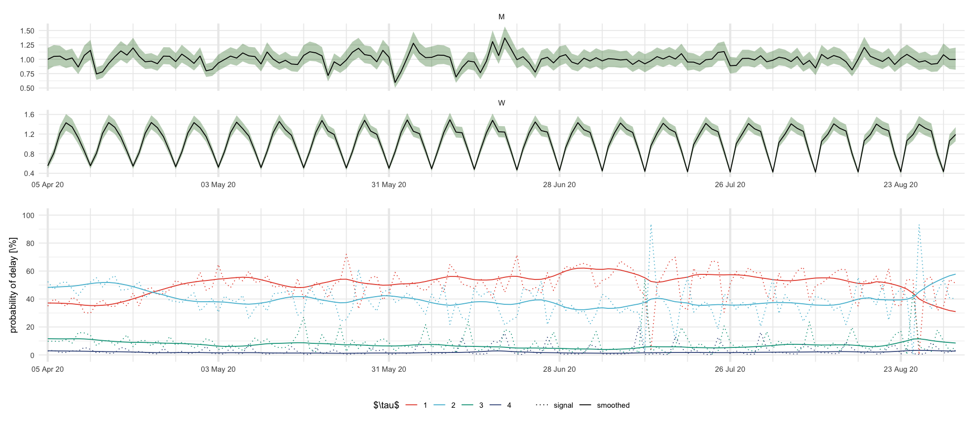
figures/showcase_prediction_intervals.tex
plt_MW <- df_showcase %>%
    filter((variable %in% c("M", "W"))) %>%
    ggplot(aes(date, mean)) +
    geom_ribbon(aes(date, ymin = `0.025`, ymax = `0.975`), fill = "darkgreen", alpha = .3) +
    geom_line() +
    facet_wrap(~variable, scales = "free_y", ncol = 1) +
    labs(x = "", y = "")

plt_p <- df_showcase %>%
    filter(str_starts(variable, "\\$p")) %>%
    mutate(delay = str_extract(variable, "\\d+")) %>%
    select(date, mean, variable, delay) %>%
    mutate(variable = ifelse(str_detect(variable, "s"), "smoothed", "signal")) %>%
    ggplot(aes(date, 100 * mean, color = delay, linetype = variable)) +
    geom_line() +
    scale_y_continuous(breaks = 20 * 0:5, limits = c(0, 1) * 100) +
    scale_linetype_manual(values = c("signal" = "dotted", "smoothed" = "solid")) +
    labs(color = "$\\tau$", x = "", y = "probability of delay [\\%]", linetype = "")

plt_MW / plt_p + plot_layout(guides = "collect") & theme(legend.position = "bottom") & scale_x_four_weekly()
# theme(axis.text.x = element_text(angle = 45, hjust = 1))
ggsave_tikz(here("tikz/showcase_prediction_intervals.tex"), height = 1.5 * default_height)
agg_record_1559631979: 2
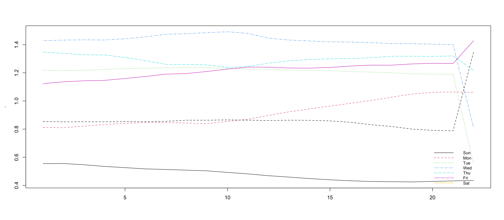
Weekday effect changes slightly over time
df_showcase %>%
    filter(variable == "W") %>%
    pull(mean) %>%
    head(-1) %>%
    matrix(nrow = 7) %>%
    t() %>%
    matplot(type = "l")
legend("bottomright", lty = 1:7, legend = c("Sun", "Mon", "Tue", "Wed", "Thu", "Fri", "Sat"), col = 1:7, cex = 0.8, bty = "n")
Warning message in matrix(., nrow = 7):
“data length [149] is not a sub-multiple or multiple of the number of rows [7]”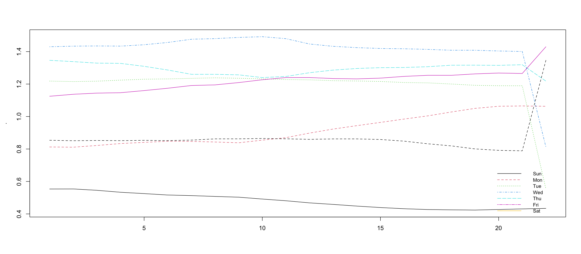
Weekly average of weekday effects close to 1
df_showcase %>%
    filter(variable == "running_W") %>%
    select(mean, sd) %>%
    head(-3) %>%
    tail(-3) %>%
summarize(mean(.$mean), mean(.$sd))| mean(.$mean) | mean(.$sd) |
|---|---|
| <dbl> | <dbl> |
| 1.057842 | 0.00642704 |
df_showcase %>%
    filter(variable == "running_W") %>%
    ggplot(aes(date, mean)) +
    geom_line() +
    geom_ribbon(aes(ymin = `0.025`, ymax = `0.975`), fill = "darkgreen", alpha = .3)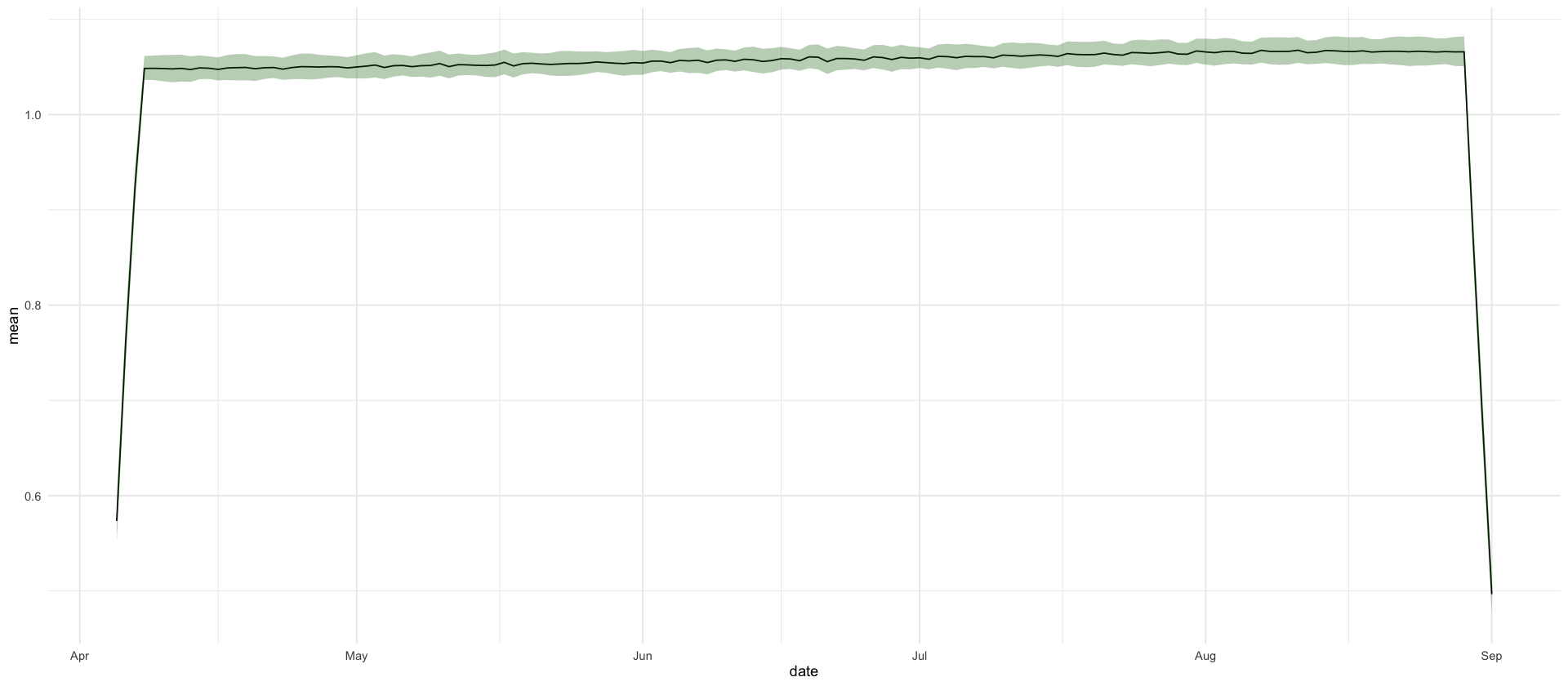
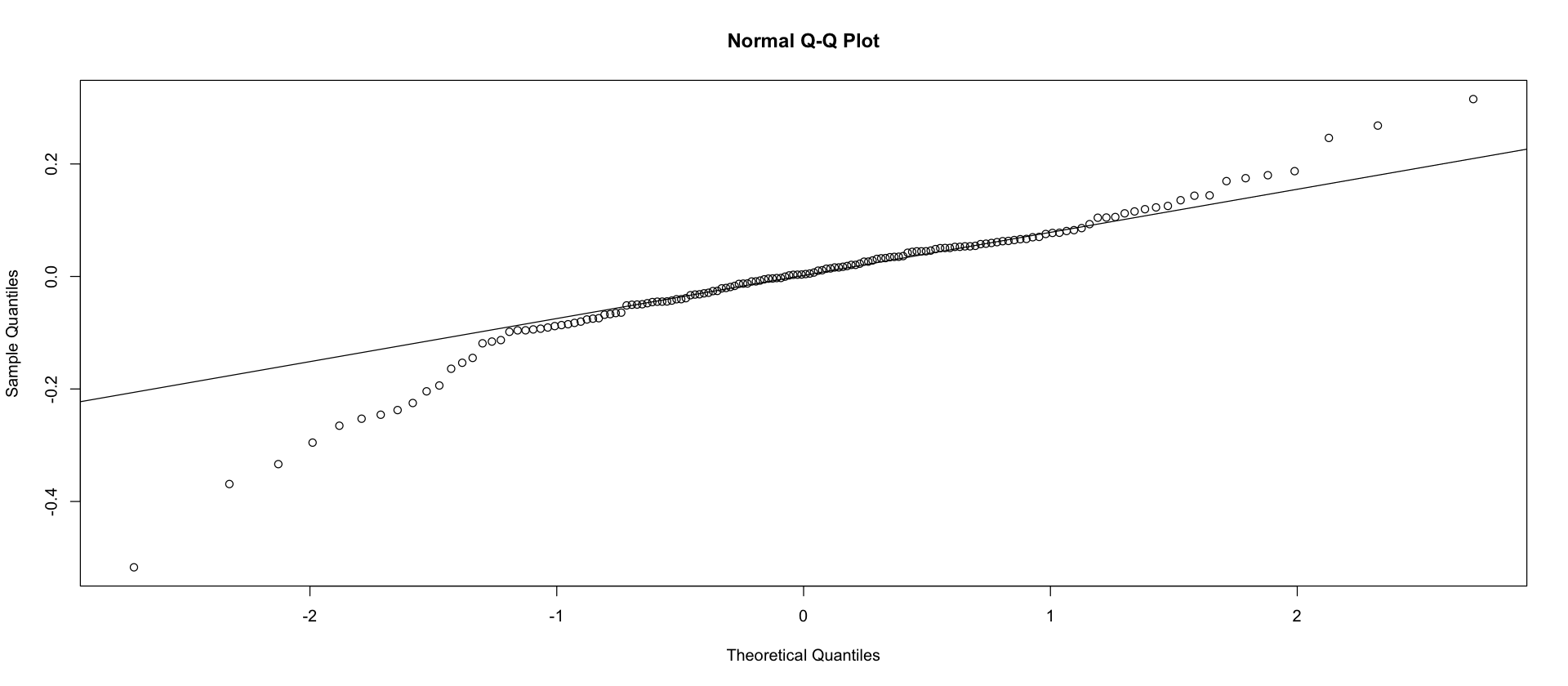
Heavier tails than normal tails in mean M.
mean_Ms <- df_showcase %>%
    filter(variable == "M") %>%
    pull(mean)

mean(mean_Ms)

qqnorm(log(mean_Ms))
qqline(log(mean_Ms))
0.999627559009596
Christmas
parameters
theta_christmas <- read_csv(here("data/results/4_christmas_model/thetas.csv")) %>%
    rename("\\rho" = 2)
theta_christmas_miss <- read_csv(here("data/results/4_christmas_model/thetas_miss.csv")) %>%
    rename("\\rho" = 2)

sds_christmas <- theta_christmas %>%
    mutate(across(where(is.numeric), ~ exp(.x / 2)))
sds_christmas_miss <- theta_christmas_miss %>%
    mutate(across(where(is.numeric), ~ exp(.x / 2)))
se <- read_csv(here("data/results/4_christmas_model/standard_errors_non_miss.csv")) %>%
pivot_wider(names_from=1, values_from=2) %>%
rename("\\rho" = 1) %>%
mutate(method = "standard_error") %>%
select(method, everything())
se_miss <- read_csv(here("data/results/4_christmas_model/standard_errors_miss.csv")) %>%
pivot_wider(names_from=1, values_from=2) %>%
rename("\\rho" = 1) %>%
mutate(method = "standard_error") %>%
select(method, everything())tables/christmas-parameters.tex
# use scientific notation
sds_concat <- sds_christmas %>%
    bind_rows(
        se,
        sds_christmas_miss,
        se_miss
    ) %>%
    rename_with(function(col) str_glue("$\\hat\\sigma_{{ {col} }}$"), where(is.numeric))
sds_concat %>%
filter(method %in% c("MLE", "standard_error")) %>%
mutate(scenario = c("all", "all", "C. rem.", "C. rem.")) %>%
pivot_longer(-c(method, scenario), names_to = "parameter", values_to = "value") %>%
pivot_wider(names_from = method, values_from = value) %>%
mutate(
lower = MLE - 2 * standard_error,
upper = MLE + 2 * standard_error
)| scenario | parameter | MLE | standard_error | lower | upper |
|---|---|---|---|---|---|
| <chr> | <chr> | <dbl> | <dbl> | <dbl> | <dbl> |
| all | $\hat\sigma_{ \rho }$ | 0.012597132 | 0.0003185590 | 0.011960014 | 0.01323425 |
| all | $\hat\sigma_{ W }$ | 0.031500111 | 0.0006740364 | 0.030152038 | 0.03284818 |
| all | $\hat\sigma_{ q }$ | 0.375075886 | 0.0505961058 | 0.273883675 | 0.47626810 |
| all | $\hat\sigma_{ M }$ | 0.110339036 | 0.0025024413 | 0.105334153 | 0.11534392 |
| all | $\hat\sigma_{ W_q }$ | 0.905485643 | 0.0470995462 | 0.811286550 | 0.99968473 |
| C. rem. | $\hat\sigma_{ \rho }$ | 0.008689361 | 0.0015244479 | 0.005640465 | 0.01173826 |
| C. rem. | $\hat\sigma_{ W }$ | 0.027744777 | 0.0015711518 | 0.024602473 | 0.03088708 |
| C. rem. | $\hat\sigma_{ q }$ | 0.160957656 | 0.0039757282 | 0.153006200 | 0.16890911 |
| C. rem. | $\hat\sigma_{ M }$ | 0.048454349 | 0.0044374841 | 0.039579381 | 0.05732932 |
| C. rem. | $\hat\sigma_{ W_q }$ | 0.376345876 | 0.0212759141 | 0.333794048 | 0.41889770 |
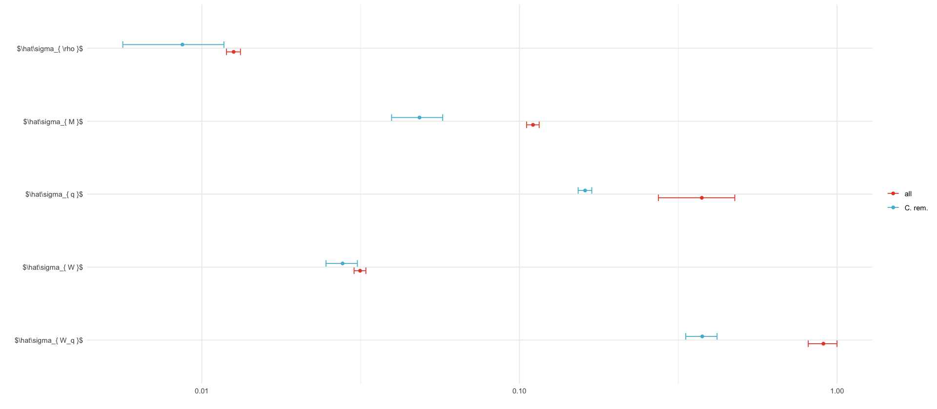
sds_concat %>%
    filter(method %in% c("MLE", "standard_error")) %>%
    mutate(scenario = c("all", "all", "C. rem.", "C. rem.")) %>%
    pivot_longer(-c(method, scenario), names_to = "parameter", values_to = "value") %>%
    pivot_wider(names_from = method, values_from = value)  %>%
    ggplot(aes(parameter, color=scenario)) +
    geom_point(aes(y=MLE), position = position_dodge2(width=.2)) +
    geom_errorbar(aes(ymin=MLE - 2* standard_error, ymax = MLE+ 2 * standard_error), position = position_dodge2(width=.1), width=.2) +
    scale_y_log10() +
    scale_x_discrete(limits = rev) +
    coord_flip() +
    labs(x="", y="", color="")

ggsave_tikz(here("tikz/christmas_parameters_CI.tex"), height=3, width=7.5)
agg_record_127092350: 2
fmt_round <- function(x, k=3) format(round(x, k), nsmall=k)

sds_concat %>%
    mutate(method = paste0(method, ifelse(1:8 < 5, "_all", "_removed"))) %>%
    pivot_longer(-method, names_to = "parameter", values_to = "value") %>%
    pivot_wider(names_from = method, values_from = value) %>%
    select(-manual_removed) %>%
    mutate(
        MLE_all_display = str_glue("{fmt_round(MLE_all)} ({fmt_round(standard_error_all)})"),
        MLE_removed_display = str_glue("{fmt_round(MLE_removed)} ({fmt_round(standard_error_removed)})")
    )  %>%
    mutate(across(where(is.numeric), fmt_round)) %>%
    select(parameter, manual = manual_all, initial_all, initial_removed, MLE_all_display, MLE_removed_display) %>%
    kable(format = "latex", booktabs = T, escape = F, col.names=c(" ", "\\textbf{manual}", "\\textbf{all}", "\\textbf{C. rem.}", "\\textbf{all}", "\\textbf{C. rem.}"), align = c("l", "c", "c", "c", "c", "c")) %>% add_header_above(
        c(" " = 2, "$\\\\theta^0$" = 2, "$\\\\hat\\\\theta$" = 2),
        escape = F, line = TRUE
    ) %>%
    cat(., file = here("tables/christmas-parameters.tex"))
Predictions
df_christmas <- read_predictions(
    here("data/results/4_christmas_model/predictions.npy"),
    seq(ymd("2020-10-01"), ymd("2021-02-28"), by = "1 day"),
    c("I", "$\\rho$", "M", "W", "running_W", "$p^s_1$", "$p^s_2$", "$p^s_3$", "$p^s_4$", "$p_1$", "$p_2$", "$p_3$", "$p_4$", "$W_{q_1}", "W_{q_2}", "W_{q_3}", "y_christmas")
)

df_christmas_missing <- read_predictions(
    here("data/results/4_christmas_model/predictions_miss.npy"),
    seq(ymd("2020-10-01"), ymd("2021-02-28"), by = "1 day"),
    c("I", "$\\rho$", "M", "W", "running_W", "$p^s_1$", "$p^s_2$", "$p^s_3$", "$p^s_4$", "$p_1$", "$p_2$", "$p_3$", "$p_4$", "$W_{q_1}", "W_{q_2}", "W_{q_3}", "y_christmas")
)
missing_indices <- 80:109
dates_missing <- sort(unique(df_christmas$date))[missing_indices]
range(dates_missing)predictive distribution of total number of cases
imputed <- df_christmas_missing %>%
    filter(variable == "y_christmas") %>%
    head(1) %>%
    select(-date, -variable) %>%
    pivot_longer(everything()) %>%
    deframe()

removed <- total_df %>%
    filter(date %in% dates_missing) %>%
    summarize(sum(total)) %>%
    pull()

f_digit <- function(x) format(round(x, -3), big.mark = ",")
str_glue("Removed {format(removed, big.mark=',')} cases")
str_glue("Mean imputed cases: {f_digit(imputed['mean'])}+- {f_digit(imputed['sd'])}, 95% PI {f_digit(imputed['0.025'])} - {f_digit(imputed['0.975'])} ")
str_glue("Median imputed cases: {f_digit(imputed['0.5'])}")
'Removed 551,031 cases'
'Mean imputed cases: 618,000+- 59,000, 95% PI 512,000 - 743,000 '
'Median imputed cases: 615,000'
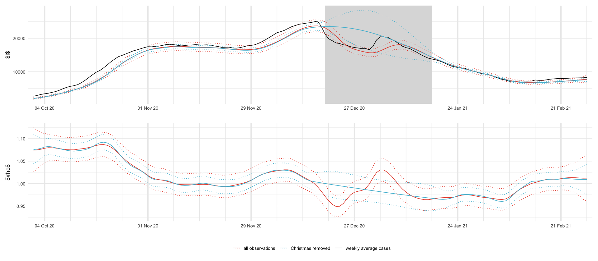
df_plot <- rbind(
    mutate(df_christmas, model = "all observations"),
    mutate(df_christmas_missing, model = "Christmas removed")
) %>%
    select(model, date, variable, mean, `0.025`, `0.975`) %>%
    filter(variable %in% c("I", "$\\rho$"))

total_df_smoothed <- total_df %>%
    mutate(total = rollmean(total, 7, 0, True, align = "center")) %>%
    filter(date %in% unique(df_plot$date)) %>%
    mutate(model = "weekly average cases")

plt_I <- df_plot %>%
    filter(variable == "I") %>%
    ggplot(aes(date, mean, color = model)) +
    geom_rect(xmin = min(dates_missing), xmax = max(dates_missing), ymin = -Inf, ymax = Inf, fill = "gray", alpha = .01, inherit.aes = F) +
    geom_line(aes(date, total), data = total_df_smoothed) +
    # geom_ribbon(aes(ymin = `0.025`, ymax = `0.975`, fill = model), alpha = .3) +
    geom_line(aes(y = `0.025`, color = model), linetype = "dotted") +
    geom_line(aes(y = `0.975`, color = model), linetype = "dotted") +
    geom_line() +
    labs(x = "", y = "$I$", fill = "", color = "") +
    scale_color_manual(values = c("all observations" = pal_npg()(3)[1], "Christmas removed" = pal_npg()(3)[2], "weekly average cases" = "black"))

plt_rho <- df_plot %>%
    filter(variable == "$\\rho$") %>%
    ggplot(aes(date, mean, color = model)) +
    # geom_rect(xmin = min(dates_missing), xmax = max(dates_missing), ymin = -Inf, ymax = Inf, fill = "gray80", alpha = .01, inherit.aes = F) +
    # geom_ribbon(aes(ymin = `0.025`, ymax = `0.975`, fill = model), alpha = .3) +
    geom_line(aes(y = `0.025`, color = model), linetype = "dotted", show.legend = F) +
    geom_line(aes(y = `0.975`, color = model), linetype = "dotted", show.legend = F) +
    geom_line(show.legend = F) +
    labs(x = "", y = "$\\rho$", fill = "", color = "")


plt_I / plt_rho + plot_layout(guides = "collect") & theme(legend.position = "bottom") & scale_x_four_weekly()

ggsave_tikz(here("tikz/christmas_prediction_intervals_I_rho.tex"))
pdf: 2
median in christmas period smaller than mean for missing model
df_christmas_missing %>%
    filter(variable == "I") %>%
    select(date, mean, `0.5`) %>%
    pivot_longer(-date) %>%
    ggplot(aes(date, value, color = name)) +
    geom_line()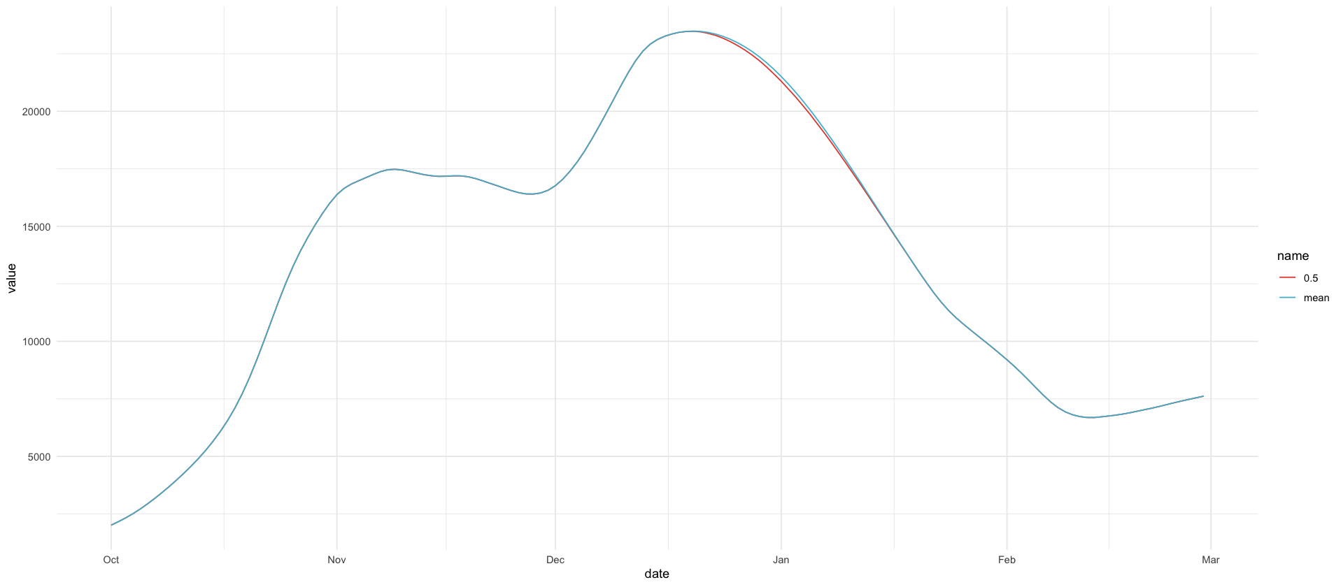
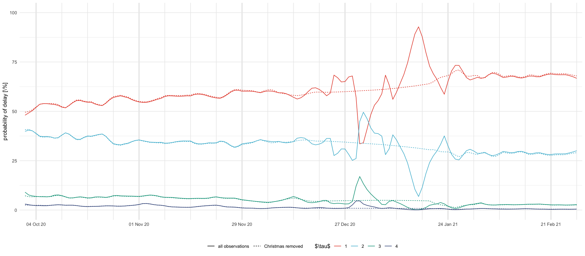
tikz/christmas_delay_probs.tex
df_plot <- rbind(
    mutate(df_christmas, model = "all observations"),
    mutate(df_christmas_missing, model = "Christmas removed")
) %>%
    select(model, date, variable, mean, `0.025`, `0.975`) %>%
    filter(str_starts(variable, "\\$p\\^s")) %>%
    mutate(delay = str_extract(variable, "\\d+")) %>%
    select(-variable)


df_plot %>%
    ggplot(aes(date, 100 * mean, color = delay, linetype = model)) +
    geom_line() +
    ylim(0, 100) +
    scale_x_four_weekly() +
    labs(x = "", y = "probability of delay [\\%]", color = "$\\tau$", linetype = "") +
    theme(legend.position = "bottom")

ggsave_tikz(here("tikz/christmas_delay_probs.tex"), height = 1 / 2 * default_height)
pdf: 2