library(here)
source(here("setup.R"))
here() starts at /Users/stefan/workspace/work/phd/thesis
library(here)
source(here("setup.R"))here() starts at /Users/stefan/workspace/work/phd/thesis
hospitalisations_raw <- read_csv(here("data/raw/all_hosp_age.csv")) %>%
    select(-location) %>%
    rename(a = age_group, s = case_date, t = hosp_date, H = value)

rki_raw <- read_csv(here("data/raw/delayed_cases_age.csv"))
# helper to summarize over age groups
sum_age_groups <- function(df, age_column = "a", value_column = "h", all_age_value = "00+") {
df %>%
group_by(across(-c(!!age_column, !!value_column))) %>%
summarize(!!value_column := sum(!!rlang::sym(value_column))) %>%
mutate(!!age_column := "00+") %>%
select(-!!age_column, -!!value_column, !!age_column, !!value_column)
}
add_all_age_groups <- function(df, age_column = "a", value_column = "h", all_age_value = "00+") {
df %>%
rbind(sum_age_groups(df, age_column, value_column, all_age_value))
}hospitalisations_raw| t | s | a | H |
|---|---|---|---|
| <date> | <date> | <chr> | <dbl> |
| 2021-04-06 | 2020-03-04 | 00-04 | 0 |
| 2021-04-06 | 2020-03-04 | 05-14 | 0 |
| 2021-04-06 | 2020-03-04 | 15-34 | 17 |
| 2021-04-06 | 2020-03-04 | 35-59 | 34 |
| 2021-04-06 | 2020-03-04 | 60-79 | 12 |
| 2021-04-06 | 2020-03-04 | 80+ | 1 |
| 2021-04-06 | 2020-03-05 | 00-04 | 0 |
| 2021-04-06 | 2020-03-05 | 05-14 | 0 |
| 2021-04-06 | 2020-03-05 | 15-34 | 17 |
| 2021-04-06 | 2020-03-05 | 35-59 | 41 |
| 2021-04-06 | 2020-03-05 | 60-79 | 16 |
| 2021-04-06 | 2020-03-05 | 80+ | 2 |
| 2021-04-06 | 2020-03-06 | 00-04 | 0 |
| 2021-04-06 | 2020-03-06 | 05-14 | 0 |
| 2021-04-06 | 2020-03-06 | 15-34 | 18 |
| 2021-04-06 | 2020-03-06 | 35-59 | 54 |
| 2021-04-06 | 2020-03-06 | 60-79 | 16 |
| 2021-04-06 | 2020-03-06 | 80+ | 4 |
| 2021-04-06 | 2020-03-07 | 00-04 | 1 |
| 2021-04-06 | 2020-03-07 | 05-14 | 3 |
| 2021-04-06 | 2020-03-07 | 15-34 | 22 |
| 2021-04-06 | 2020-03-07 | 35-59 | 74 |
| 2021-04-06 | 2020-03-07 | 60-79 | 26 |
| 2021-04-06 | 2020-03-07 | 80+ | 9 |
| 2021-04-06 | 2020-03-08 | 00-04 | 1 |
| 2021-04-06 | 2020-03-08 | 05-14 | 3 |
| 2021-04-06 | 2020-03-08 | 15-34 | 25 |
| 2021-04-06 | 2020-03-08 | 35-59 | 81 |
| 2021-04-06 | 2020-03-08 | 60-79 | 35 |
| 2021-04-06 | 2020-03-08 | 80+ | 9 |
| ⋮ | ⋮ | ⋮ | ⋮ |
| 2023-12-19 | 2023-12-15 | 00-04 | 316 |
| 2023-12-19 | 2023-12-15 | 05-14 | 52 |
| 2023-12-19 | 2023-12-15 | 15-34 | 395 |
| 2023-12-19 | 2023-12-15 | 35-59 | 1116 |
| 2023-12-19 | 2023-12-15 | 60-79 | 3344 |
| 2023-12-19 | 2023-12-15 | 80+ | 4174 |
| 2023-12-19 | 2023-12-16 | 00-04 | 309 |
| 2023-12-19 | 2023-12-16 | 05-14 | 53 |
| 2023-12-19 | 2023-12-16 | 15-34 | 371 |
| 2023-12-19 | 2023-12-16 | 35-59 | 1048 |
| 2023-12-19 | 2023-12-16 | 60-79 | 3243 |
| 2023-12-19 | 2023-12-16 | 80+ | 4040 |
| 2023-12-19 | 2023-12-17 | 00-04 | 304 |
| 2023-12-19 | 2023-12-17 | 05-14 | 53 |
| 2023-12-19 | 2023-12-17 | 15-34 | 367 |
| 2023-12-19 | 2023-12-17 | 35-59 | 1049 |
| 2023-12-19 | 2023-12-17 | 60-79 | 3205 |
| 2023-12-19 | 2023-12-17 | 80+ | 4004 |
| 2023-12-19 | 2023-12-18 | 00-04 | 305 |
| 2023-12-19 | 2023-12-18 | 05-14 | 54 |
| 2023-12-19 | 2023-12-18 | 15-34 | 362 |
| 2023-12-19 | 2023-12-18 | 35-59 | 1037 |
| 2023-12-19 | 2023-12-18 | 60-79 | 3160 |
| 2023-12-19 | 2023-12-18 | 80+ | 3957 |
| 2023-12-19 | 2023-12-19 | 00-04 | 240 |
| 2023-12-19 | 2023-12-19 | 05-14 | 43 |
| 2023-12-19 | 2023-12-19 | 15-34 | 283 |
| 2023-12-19 | 2023-12-19 | 35-59 | 807 |
| 2023-12-19 | 2023-12-19 | 60-79 | 2543 |
| 2023-12-19 | 2023-12-19 | 80+ | 3076 |
reporting_triangle_processed <- hospitalisations_raw %>%
mutate(delay = as.numeric(t - s)) %>%
# d = 0 is known, chunk remainder into weekly units
mutate(k = (delay + 5) %/% 7) %>%
group_by(s, a, k) %>%
summarize(H = max(H)) %>%
filter(k < 8) %>%
arrange(s, k) %>%
group_by(s) %>%
# only those dates where all k are available
filter(min(k) == 0, max(k) >= 7) %>%
ungroup() %>%
group_by(s, a) %>%
arrange(k) %>%
# ensure positive increments, treat last H as truth
mutate(h = diff(c(0, pmin(cummax(H), tail(H, 1))))) %>%
ungroup() %>%
arrange(s, k) %>%
select(s, a, k, h) %>%
add_all_age_groups()
reporting_triangle_processed %>%
head()
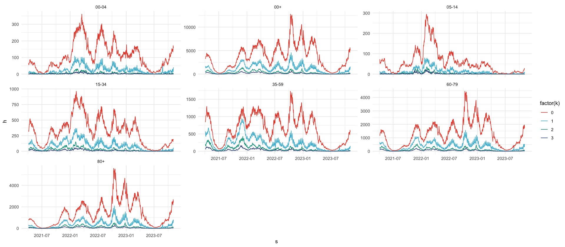
reporting_triangle_processed %>%
filter(k <= 3) %>%
ggplot(aes(s, h, color = factor(k))) +
geom_line() +
facet_wrap(~a, scale = "free_y")| s | a | k | h |
|---|---|---|---|
| <date> | <chr> | <dbl> | <dbl> |
| 2021-04-05 | 00-04 | 0 | 65 |
| 2021-04-05 | 05-14 | 0 | 73 |
| 2021-04-05 | 15-34 | 0 | 331 |
| 2021-04-05 | 35-59 | 0 | 839 |
| 2021-04-05 | 60-79 | 0 | 1160 |
| 2021-04-05 | 80+ | 0 | 778 |
reporting_triangle_processed %>%
    filter(h < 0)
stopifnot(all(reporting_triangle_processed$h >= 0))| s | a | k | h |
|---|---|---|---|
| <date> | <chr> | <dbl> | <dbl> |
seven_day_incidence_frozen <- rki_raw %>%
filter(age_group != "unbekannt") %>%
mutate(age_group = str_replace_all(age_group, "A", "")) %>%
# watch out here, aggregate seven day I by rki date, not county date?
mutate(delay = rki_date - county_date) %>%
group_by(age_group, rki_date) %>%
filter(delay <= 7) %>%
summarize(cases = sum(cases)) %>%
rename(a = age_group, s = rki_date, I = cases) %>%
add_all_age_groups(value_column = "I")
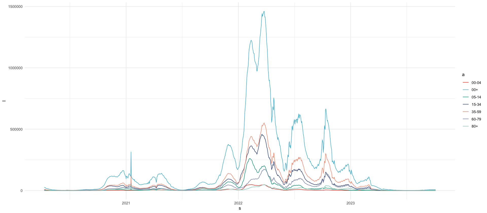
seven_day_incidence_frozen %>%
head()
seven_day_incidence_frozen %>%
ggplot(aes(s, I, color = a)) +
geom_line()| a | s | I |
|---|---|---|
| <chr> | <date> | <dbl> |
| 00-04 | 2020-04-10 | 248 |
| 00-04 | 2020-04-11 | 225 |
| 00-04 | 2020-04-12 | 219 |
| 00-04 | 2020-04-13 | 214 |
| 00-04 | 2020-04-14 | 206 |
| 00-04 | 2020-04-15 | 165 |
full_df <- reporting_triangle_processed %>%
    inner_join(seven_day_incidence_frozen)

full_df %>%
    write_csv(here("data/processed/seven_day_H_I_by_age.csv"))

full_df %>%
    head()
Joining with `by = join_by(s, a)`
| s | a | k | h | I |
|---|---|---|---|---|
| <date> | <chr> | <dbl> | <dbl> | <dbl> |
| 2021-04-05 | 00-04 | 0 | 65 | 4348 |
| 2021-04-05 | 05-14 | 0 | 73 | 9740 |
| 2021-04-05 | 15-34 | 0 | 331 | 31851 |
| 2021-04-05 | 35-59 | 0 | 839 | 41889 |
| 2021-04-05 | 60-79 | 0 | 1160 | 14813 |
| 2021-04-05 | 80+ | 0 | 778 | 3617 |